


How Uber Surge Pricing Algorithm Works: ML, Supply-Demand Modeling, and Real-Time Pricing
When 200 riders open their Uber app at Friday 11 PM outside Madison Square Garden and only 50 drivers are nearby, what happens next? Most people think: “prices go up.” What actually happens: millions of GPS coordinates stream through Apache Kafka, get bucketed into hexagonal geo-cells, trigger LSTM-based demand forecasts, and output a surge multiplier—all within 300 milliseconds.
Uber Surge pricing algorithm is not a slider in an admin panel. It is a distributed systems problem — real-time supply/demand tracking across hexagonal geo-cells, streamed through Kafka pipelines, aggregated by geo-sharded services, and served to the app within seconds. Uber surge pricing algorithm ML models are the engine behind one of the most sophisticated real-time marketplace equilibrium solutions in existence.
Who this is for:
ML engineers, data scientists, and backend engineers building pricing systems, recommendation engines, or any real-time prediction infrastructure that needs to process millions of events per second.
What you’ll understand:
The actual technical architecture—not marketing fluff, not hand-waving, but the models, the data pipelines, the distributed systems patterns, and the ML infrastructure that powers Uber’s $31.8B pricing engine.
Table of Contents
The Geospatial Foundation: Why Hexagons, Not Squares
Here’s the problem every location-based ML system faces: you need to aggregate GPS coordinates—millions of them, updating every 4 seconds—into discrete spatial buckets where you can compute supply, demand, and ultimately price. The naive approach is to use square grids (latitude/longitude tiles). Uber tried that. It doesn’t work.
Why square grids fail:
Square grid cells have a fundamental geometric problem: the distance from a cell center to its corners is 1.41x the distance to its edges. When you’re trying to compute “how many drivers are within 5 minutes of this pickup point,” that 41% distance variance creates massive edge effects. A driver 10 meters over a cell boundary might be the closest available driver, but your aggregation logic doesn’t see them because they’re in a different bucket.
Zoom levels do not nest cleanly. Aggregating from small cells to larger cells in a square grid introduces edge artifacts. Cell boundaries cross natural features like rivers and highways in ways that do not match real-world travel patterns.
Enter H3: Uber’s hexagonal hierarchical spatial index
Uber developed H3, an open source grid system for optimizing ride pricing and dispatch. Data points are bucketed into hexagons and can be written using the hexagonally bucketed data. For example, surge pricing is calculated by measuring supply and demand in hexagons in each city.
H3 divides the entire planet into hexagons at 16 different resolutions. Each hexagon has a 64-bit identifier that encodes both location and resolution. At resolution 9 (typical for city-level surge pricing), each hexagon covers approximately 0.1 square kilometers. At resolution 7, hexagons span about 5 square kilometers—useful for regional demand patterns.
Why hexagons are superior for ML:
1. Uniform neighbor distances: Every hexagon has 6 neighbors, and the distance from any hexagon center to all 6 neighbor centers is identical. This eliminates quantization error when users move through a city. In ML terms, your spatial features have consistent geometric properties.
2. Hierarchical aggregation: H3 uses a hierarchical structure where every hexagon at resolution N contains exactly 7 hexagons at resolution N+1. This makes multi-scale feature engineering trivial—you can compute demand at the block level, neighborhood level, and city level using the same index structure.
3. Efficient radius queries: “Find all drivers within 10 hexagons” becomes a simple graph traversal. No complex spatial joins, no bounding box calculations. You’re working with discrete cell IDs, not continuous coordinates.
16
64-bit
0.1 km²
4 sec
How this impacts the pricing model:
When you open the Uber app, the pricing service needs to know: what’s the supply-demand ratio in your hexagon right now? Not your exact GPS coordinate—your hexagon. This is a lookup, not a computation. The surge multiplier has already been calculated for hex ID 8928308280fffff (that’s an actual H3 identifier for a hexagon in San Francisco’s Mission District). The app just fetches it.
The entire streaming pipeline is built around this: driver GPS updates get mapped to hex IDs, rider requests get mapped to hex IDs, and the aggregation logic counts events per hex. No spatial joins. No distance calculations. Just: group_by(hex_id) → compute supply/demand ratio → output surge multiplier.
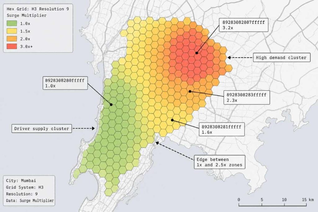
H3 hex grid overlay on Mumbai map visualizing surge pricing clusters and demand–supply zones.
Real-Time Demand Forecasting with LSTM Networks
Surge pricing isn’t purely reactive. If Uber waited until demand spiked before raising prices, riders would see availability drop to zero before surge kicked in. The system needs to predict demand 15-30 minutes into the future so it can adjust prices proactively.
This is where recurrent neural networks come in—specifically, Long Short-Term Memory (LSTM) networks.
Why time-series forecasting is hard for Uber
At Uber, event forecasting enables prediction of where, when, and how many ride requests Uber will receive at any given time. Extreme events—peak travel times such as holidays, concerts, inclement weather, and sporting events—heighten the importance of forecasting.
Traditional time-series methods like ARIMA assume stationary processes with predictable seasonality. Uber’s demand patterns are anything but stationary: a concert lets out at 10:15 PM and suddenly 5,000 people need rides from one location. A rainstorm starts, and demand spikes 200% citywide in 10 minutes. These are the “extreme events” where accurate forecasting has the highest business impact—and where classical methods fail.
LSTM architecture for demand prediction
The model uses Long Short Term Memory (LSTM) architecture, a technique that features end-to-end modeling, ease of incorporating external variables, and automatic feature extraction abilities.
Here’s what the model actually learns:
Input sequence (per hexagon):
- Historical demand: ride requests per 5-minute window, last 2 hours (24 time steps)
- Driver supply: available drivers per 5-minute window, last 2 hours
- Completion rate: % of requests matched to drivers, last 2 hours
- External features: weather conditions, time of day, day of week, local events flag
Output: Predicted ride requests for next 30 minutes (6 time steps, 5 minutes each)
The LSTM encoder-decoder processes this input sequence through stacked LSTM layers (typically 2-3 layers, 128-256 hidden units per layer). The model learns to identify patterns like: “When completion rate drops below 85% and it starts raining, demand typically increases 40% in the next 15 minutes.”
Key technical challenges Uber solved:
1. Multi-scale forecasting: You can’t train one LSTM per hexagon—that’s millions of models. But training a single model on all hexagons produces poor results because demand patterns in Manhattan look nothing like patterns in suburban Phoenix. Solution: Meta-learning approach where the model learns city-level embeddings. The LSTM takes as input: [hexagon_features, city_embedding_vector]. This lets the model generalize patterns across cities while adapting to local characteristics.
2. Handling sparse data: Many hexagons have zero rides in a given 5-minute window. This creates extremely sparse input sequences. The model uses weighted loss functions that penalize errors on non-zero predictions more heavily than errors on zero predictions.
3. Uncertainty estimation: A point forecast (“we predict 47 rides”) isn’t useful for pricing decisions. You need confidence intervals. Uber implemented a Bayesian LSTM that outputs prediction distributions, not point estimates.
How forecasts drive pricing decisions:
The forecasting model runs continuously, outputting predictions every 5 minutes for every hexagon. These predictions feed into the pricing model as features:
predicted_demand_next_15minpredicted_supply_next_15mindemand_trend(increasing, stable, decreasing)forecast_confidence(prediction uncertainty)
When the model predicts rising demand with high confidence, the pricing engine can activate surge earlier—smoothing the demand curve rather than letting it spike and crash.
Ride Requests per Hexagon Over Time
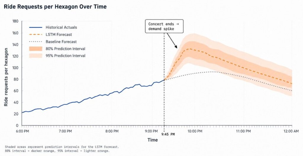
Around 9:45 PM, a large concert in the city wraps up, and thousands of attendees exit the venue almost simultaneously. As people begin looking for ways to get home, a significant portion of them open Uber and request rides at the same time. This sudden, concentrated burst of demand causes a sharp spike in ride requests across nearby hexagons.
Before this moment, the demand trend is relatively steady, gradually increasing through the evening as part of normal urban movement. However, the end of the concert acts as a trigger that disrupts this pattern, creating a short but intense surge in activity. After the initial rush is absorbed—typically over the next 30–60 minutes—the demand starts to stabilize and slowly decline as the crowd disperses and fewer new ride requests come in.
The graph captures this behavior clearly. The solid blue line, representing actual ride demand, shows a noticeable jump immediately after 9:45 PM, reflecting the real-world spike caused by the event. The dashed orange line, which is the LSTM-based forecast, closely tracks this increase, indicating that the model has learned to anticipate such event-driven surges.
In contrast, the dotted gray line (baseline forecast) rises more gradually and fails to capture the magnitude of the spike, since it relies on typical patterns and does not account for sudden external events. Surrounding the LSTM forecast are shaded prediction bands (80% and 95%), which widen around the spike, highlighting increased uncertainty during unpredictable, high-variance periods.
Overall, the visualization demonstrates how external events like a concert ending can dramatically influence ride demand, and why advanced forecasting models are necessary to capture these dynamics accurately.
The Pricing Decision Engine: Gradient Boosted Trees
The forecasting model predicts what will happen. The pricing model decides what price to show. These are separate ML problems requiring different architectures.
For the pricing decision itself, Uber’s surge pricing algorithm depends on regression analysis tools to determine which locations will be the busiest to activate surge pricing. This can also be used to send more drivers to that location to offer more customer-oriented services.
Why gradient boosted decision trees (GBDT), not neural networks?
The pricing model needs to be:
- Interpretable: Pricing is regulated. You need to explain why surge is 2.5x, not 2.8x.
- Fast: < 50ms inference time per request. Neural networks are overkill.
- Robust to distribution shift: Demand patterns change constantly. Tree-based models handle this better than deep learning.
GBDT models (XGBoost, LightGBM) excel at structured feature learning and handle mixed data types (continuous, categorical, sparse) without extensive preprocessing.
Feature engineering for the pricing model
The model doesn’t just see “50 drivers, 200 riders.” It sees a rich feature vector per hexagon:
Supply features:
available_drivers_count(current)available_drivers_rolling_5min(smoothed short-term trend)available_drivers_rolling_30min(broader trend)driver_utilization_rate(% of drivers on trips)driver_eta_percentile_50(median ETA from drivers to this hex)driver_eta_percentile_90(worst-case ETA
Demand features:
open_requests_count(unfulfilled ride requests)request_rate_5min(requests per minute, recent)request_rate_30min(requests per minute, broader window)forecasted_demand_15min(from LSTM model)demand_volatility(standard deviation of recent requests)
External context features:
time_of_day_binned(categorical: early_morning, morning_rush, midday, evening_rush, night)day_of_week(categorical)is_holiday(binary)weather_condition(categorical: clear, rain, snow, severe)event_flag(binary: major event happening in this hex?)airport_proximity(distance to nearest airport in hex counts)
Spatial features:
neighbor_surge_mean(average surge multiplier in adjacent hexagons)neighbor_surge_max(highest surge in adjacent hexagons)hex_density_category(urban_core, urban, suburban, rural)
Target variable: optimal_surge_multiplier (continuous, range 1.0 to 5.0)
The model learns complex interactions:
“When driver_utilization_rate > 0.90 AND forecasted_demand_15min > 1.5x current AND weather = rain → predict surge_multiplier = 2.3x”
Real-time inference architecture
The pricing algorithm processes millions of location updates every second using Apache Kafka, Apache Flink, and Redis/Memcached.
Here’s the data flow:
-
1. Event stream:
Driver GPS updates (every 4 seconds) and ride requests stream into Kafka topics, partitioned by city.
-
2. Feature computation:
Apache Flink jobs consume these streams, aggregate events by hex ID, compute rolling statistics, and write features to Redis (in-memory cache).
-
3. Model serving:
When a rider opens the app, the API service:
- Maps rider location → hex ID (< 1ms)
- Fetches features for that hex from Redis (< 5ms)
- Calls model inference service with feature vector (< 20ms)
- Returns surge multiplier to mobile app
-
4. Total latency:
Typically 30-50ms. The entire decision—from “user opened app” to “show 2.2x surge”—happens faster than a human eye blink.
<1ms
<5ms
<20ms
~50ms
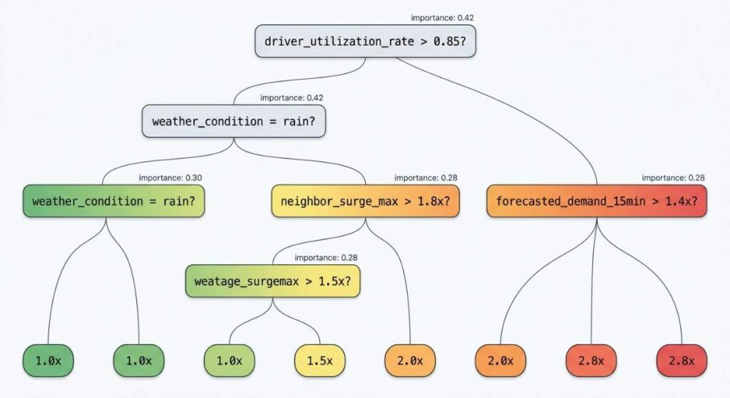
A decision tree model with a target surge multiplier of 2.8x
Here is a decision tree illustrating how a machine learning model might determine surge pricing in real-time. It starts by assessing the critical variable of driver availability, then factors in external conditions like rain, and finally considers localized demand pressures to assign an optimal fare multiplier. This dynamic logic ensures that pricing remains responsive to both immediate and forecasted imbalances between rider demand and driver supply.
Feature Engineering at Scale: The Michelangelo Platform
Machine learning models are only as good as their features. At Uber’s scale, feature engineering isn’t just writing Pandas code—it’s a distributed systems problem.
The dual-pipeline challenge
Every ML feature needs to be computed in two completely different contexts:
1. Offline (training time): You’re processing historical data in Spark, joining massive datasets in Hive, aggregating billions of events. Time doesn’t matter. Accuracy matters.
2. Online (inference time): You have 20 milliseconds to compute features and return a prediction. You can’t run Spark queries. You can’t join 5 tables. You need features pre-computed and cached.
This is called the train-serve skew problem: if your training pipeline computes features differently than your serving pipeline, your model performance in production will degrade.
Michelangelo’s solution: Feature Store (Palette)
Michelangelo consists of a mix of open source systems and components built in-house. The primary open sourced components used are HDFS, Spark, Samza, Cassandra, MLLib, XGBoost, and TensorFlow.
The Feature Store provides a unified API where data scientists define features once, and the platform automatically generates both batch and streaming pipelines.
Example: "Average driver ETA in this hexagon over last 30 minutes"
feature {
name:”driver_eta_hex_mean_30min”
entity: “hexagon_id”
aggregation: MEAN
window: 30_MINUTES
source:driver_location_stream
field: eta_seconds
}
What Michelangelo generates:
1. Offline pipeline (Spark): Reads driver_location_stream from HDFS (historical data), Groups by hexagon_id, computes rolling 30-minute mean of eta_seconds, Writes output to training dataset
2. Online pipeline (Samza): Subscribes to driver_location_stream Kafka topic (real-time), Maintains sliding 30-minute windows per hexagon_id in stateful memory, Writes computed values to Cassandra (low-latency key-value store), Model serving containers read from Cassandra at inference time
How features scale to millions of predictions/second
Michelangelo currently powers roughly 1 million predictions per second. To enable highly efficient model serving, models and library dependencies are loaded into and served from memory.
The serving architecture uses in-memory caching aggressively:
- Model parameters: Loaded into RAM once per deployment (GBDT models are typically 50-200 MB).
- Feature values: Cached in Redis/Memcached with sub-millisecond lookup times.
- Precomputed surge multipliers: For the 95% of cases where supply/demand hasn’t changed significantly in the last minute, serve a cached multiplier. Only recompute when thresholds are crossed.
This multi-tier caching strategy reduces average inference latency from ~100ms (cold path: compute all features, run model) to ~15ms (warm path: fetch cached features, run model) to ~2ms (hot path: serve cached prediction).
Conclusion: The Stack That Keeps Surge Pricing Under 300ms
The Uber surge pricing algorithm ML ecosystem represents a pinnacle of operational research and high-scale engineering. By moving beyond simple reactive pricing and implementing predictive, spatiotemporal models, the system ensures that the marketplace remains liquid even during extreme volatility.
For the data scientist or ML engineer, the architecture serves as a blueprint for handling the complexities of a two-sided marketplace:
Data Granularity: Using H3 hexagonal indexing to prevent data dilution across large areas.
Anticipatory Intelligence: Utilizing LSTM and GRU networks to model demand before it manifests as a request.
Incentive Alignment: Applying reinforcement learning to understand the price elasticity of independent supply agents.
While surge pricing is often viewed through the lens of cost, its technical reality is one of reliability. It is the difference between a ride that is expensive but available, and a service that is unavailable at any price. As these algorithms continue to evolve with more sophisticated smoothing techniques and real-time processing, they set the standard for how we manage the physical world through digital intelligence.
Read more: Anticipatory Intelligence
What this means for your career
If you’re working on pricing systems, recommendation engines, or any real-time ML application, you’re solving similar problems: streaming data ingestion, feature engineering at scale, low-latency inference, model monitoring in production. The patterns here—hexagonal spatial indexes, LSTM forecasting → GBDT decision models, dual batch/stream pipelines—transfer directly.
The surge pricing algorithm isn’t just about ride-hailing. It’s a blueprint for building industrial-strength real-time ML systems. Every ride, every price, every prediction is a small miracle of distributed computing, machine learning, and systems engineering working in concert.
Frequently Asked Questions
What is the primary goal of the Uber surge pricing algorithm ML?
The core objective is to ensure marketplace reliability by balancing supply and demand in real-time<!–>–>. It functions as both a throttle for excess demand and an incentive for drivers to move into high-need areas<!–>–>.
Why does Uber use hexagonal H3 grids instead of square grids?
Uber utilizes the H3 hexagonal indexing system because the distance between the center of a hexagon and all its neighbors is constant. This uniformity is critical for ML models to accurately calculate and predict supply movement across a city.
How does the algorithm predict demand before it happens?
The system employs Deep Learning models, such as LSTMs and GRUs, to analyze historical patterns, weather, and real-time “latent demand” signals like app opens. This allows the algorithm to identify potential spikes before riders even press the request button.
What prevents surge prices from varying wildly between adjacent blocks?
The algorithm applies spatiotemporal smoothing to ensure price consistency. This prevents “boundary effects” where a rider might walk a short distance to find a significantly lower price, which would disrupt the equilibrium of the neighboring cell.
How does Uber determine if a price increase will actually bring in more drivers?
The algorithm estimates the price elasticity of supply using Multi-Armed Bandit frameworks and Reinforcement Learning. These models help determine the minimum multiplier required to incentivize enough drivers to reach a specific area and reduce ETAs.